Prerequisites

• DP optimization notions

Abstract

The scope of this article is presenting a very useful DP optimization technique, introduced in the problem Aliens at IOI 2016. The techinque is used to reduce dimensions in particular DP configurations, by exploiting the convex nature of some cost functions. We will introduce the technique by starting with a simpler DP problem, show the optimization from $O(N^2)$ to $O(Nlog\text{VAL})$, then reveal the full solution of the original problem. Apparently, the official name of this optimization technique is "parameter search" and the Chinese call it "bqs binary search".

A problem example

You are given an array $v$ of (possibly negative) integers of length $N$ ($\le 10^5$) and a number $K$ ($\le N$). Select at most $K$ disjoint subarrays of the initial sequence such that the sum of the elements included in the subarrays is maximized. The standard approach to such a problem would be a DP of the form:

Implementing this recurrence directly would be $O(N^4)$, supposing that $K$ is comparable in size to $N$. It is left as an exercise to the reader prefferably at least capable to solve a div2 C problem to find a way of optimize this recurrence to $O(N^2)$. The trick behind the "aliens optimization" is that we can add a cost (penalty) which we will denote by $\lambda$ for each taken subarray. If $\lambda=0$ the solution would be taking a subarray for each positive element, but by increasing the value of $\lambda$, the optimum solution shifts to taking fewer subarrays. Now we just have to find a $\lambda$ that allows us to take as many subarrays as possible, but still fewer that $K$. To do a small recap, $\lambda$ is the cost we assign to adding a new subarray, and increasing $\lambda$ will decrease the number of subarrays in an optimal solution or keep it the same, but never increase it. That suggests that we could just binary search the smallest value of $\lambda$ that yeilds an optimal soltion with less than $K$ elements.

Besides just the dp, we will store another auxiliary array:

These recurrences are implementable in $O(N)$, but I won't go into detail, as the target audience of this article is supposed to be able to solve this on its own. The pseudocode of the solution would look like this:

Proof and Formal Requirements

In the case of our initial problem, the fact that increasing $\lambda$ never increases the number of subarrays taken was probably a very intuitive fact, but we'd like to find an actual proof that this works and find a general criterion for using the peak setting optimization in reducing DP dimensions. This criterion is in a way concavity (or convexity). Let's denote by $\text{ans[k]}$ the answer for the problem, but using exactly $k$ subarrays. The key observation in proving that our solving method is correct is that the $\text{ans[k]}$ sequence is concave, that is $\text{ans[k]} - \text{ans[k - 1]} \le \text{ans[k - 1]} - \text{ans[k - 2]}$. A more natural way of thinking about this and the actual way most people "feel" the concavity/convexity is by interpreting it as if I have $k$ subarrays and add another one, it will help me more than if I had $k+1$ subarrays and added one more. Now let's see how this concavity helps us prove the correctness of our solution! Suppose $\lambda=0$. Our solution will just find the global maximum of our concave sequence, be it $\text{ans[p]}'$. Notice that no matter the value of $\lambda$, the fact that our sequence is concave won't change. Let's shift our attention for a bit from concave sequences to concave functions. $f(x)=\lambda x-x^2$ is a fine example. By changing $\lambda$, we can move the peak of the function wherever we want and the function will remain concave. Now let's go back to our more "discrete" sequence. We have an algorithm that finds $p$ and $\text{ans[p]}$ such that $\text{ans[p]}$ is the maximum of the sequence, but we don't want the maximum of the sequence, we want $\text{ans[k]}$ for some given $k$. So... we can force $k$ to be the maximum of the sequence, by adding a linear function to our sequnce ($\text{ans[k]} \rightarrow \text{ans[k]} + \lambda k$), just as we changed the peak of our continous function, which is exactly what we did in our solution. The algorithm will yield that the maximum of the sequence is at $k$ with the value $\text{ans[k]}+\lambda k$ and we just need to substract $\lambda k$ to obtain our desired value: $\text{ans[k]}$.

As for the general criterion, you might have already guessed it: if $(\text{ans[k]})_{1 \le k \le n}$ is the sequence of answers for given $k$s, the sequence must be convex or concave, that is:

Reconstruction Issues

Let's get back to our initial problem (there are $N$ integers, you have to choose $K$ subarrays, yada yada, blah blah) and let's change the statement, instead of selecting at most $K$, you have to select exactly $K$ subarrays. The difference is quite subtle, and the actual result is different iff there are less than $K$ non-negative integers in the sequence. In this case, we just have to replace return dp[n] - λ * aux[n] with return dp[n] - λ * k. This may seem weird and quite unintuitive as for why it works. Let's look at a few proprieties of our algorithm. First of all, it may not be the case that for each $k$ we have a corresponding set of $\lambda$s, that is: if for a given $p$, the maxium $\lambda$ for which taking $p$ objects is optimal, then the solution for $\lambda \leftarrow \lambda + \varepsilon$ where $\varepsilon$ is an arbitrarily small value, may use more than $p + 1$ objects, i.e. there may be no choice of $\lambda$ for which the optimal solution employs a fixed number of elements. This may seem as a small game-killer for our technique, but let's look at the cause of this issue. Looking back at the Proof paragraphs, we are given the condition:

In case of equality here, we may have the following situation:

If the $\lambda$ we choose equals $t$, then all of these solutions will seem equivalently good. In fact, if a subarray of solutions $\text{ans[a]}, \text{ans[a + 1]}, \dots, \text{ans[b]}$ for an arithmetic progression, there is no choice of $\lambda$ that finds any other optimal solution other than using $a$ or $b$ objects. However, the fact that our solution fails on possible arithmetic progressions from our sequence (i.e. if the sequence is not strictly convex) is the very thing that will help us solve this issue. Suppose we find the smallest lambda that makes the solution employ $\le k$ objects (let's say it uses $a$ objects). This means the answer using exactly $p$ objects is $\text{dp[p]}-\lambda p$, but this basically implies that between $p$ and $k$ (the fixed number of objects we want to use) there is an arithmetic progression (i.e. $\text{ans[k]} = \text{ans[p]} + t(k - p)$). So if the answer for $p$ would be $\text{dp[n]}-p \lambda$, then the answer for $k$ must be $\text{dp[n]}-p\lambda-(k-p)\lambda=\text{dp[n]}-\lambda k$. This is quite weird as by finding a solution for $p$, we also find the answer for $k$, even if $(\text{aux[n]}=p) \neq k$. The downside of this workaround, is that even if we can find the value of the answer, a general method of reconstructing the solution (finding out what subarrays should we select) probably doesn't exist.

Integral Lambda Search

Convex hull illustration

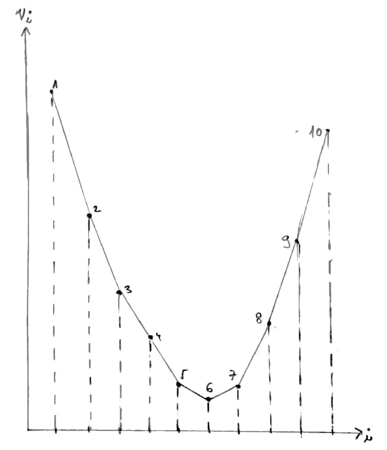
You might have noticed that we are binary searching a floating point $\lambda$, not an integral valued one. The reason is that if the prerequisites of applying the optimization are satisfied, then we have proved that a $\lambda$ exists, not that it would have an integral value. The thing is, in most DP problems, the optimization works just as well with integers. It's just not that obvious to prove why.

Let's consider a convex sequence of $N$ elements, call it $V_{1 \dots N}$. Now let's consider a set of points $P = \{ p_i=(i, v_i) | i \in [1 \dots N] \}$, once drawn, together with the line segments between consecutive points (which will bear great importance in the following steps), you will see a convex lower/upper hull. A key observation now is that when looking at our convex sequence geometrically, the "peak" of the sequence will be the unique point that has segments with different signs of the slope to its left and to its right (with the exception the edge cases where the optimum is the first or last element of the sequence). In our drawn example, that peak is the 6th point, with a segment with negative slope value on its left and positive on its right. Another useful observation is that if we have two lines $a_1 x + b_1$ and $a_2 x + b_2$, adding a constant value $\lambda$ to both their slopes doesn't change the x coordinate of their intersection:

In our context, this means that if we add a constant value to all the slopes of the segments, the intersection points will remain the same, so the peak x coordinate will still be integral. Now all that is left to do is "say" this: if we want to force a position $t$ to be the global optimum of this sequence and the slope of the segment to the left of the point is $l$ and the slope of the segment right of the point is $r$ and $\{l, r\} \subset \mathbb{Z}$, then there exists at least one value $\lambda \in \mathbb{Z}$ such that $l + \lambda$ and $r + \lambda$ have different signs. Translating this directly into terms of our convex sequence of answers, where our "slopes" are just the differences between two adjacent answers (i.e. $\text{slope[k]} = \text{ans[k + 1]} - \text{ans[k]}$), if the values of $\text{ans}$ are integral, then obviously the differences (slopes) will also be integral, so if the answers to our problem are integral, then we can always binary search $\lambda$ as an integral value.

Aliens

I find it quite amusing that when the IOI introduces some totally new technique for 99% of its contestants (like the convex hull trick with the problem batch scheduling at IOI 2002), the technique is usually merely a subproblem of a task that is quite difficult on its on own, even without the fact that the contestant is required to rediscover some then obscure technique. So is the case with Aliens (IOI 2016), even if you know the optimization, it's still quite a tricky convex hull trick problem. The solution goes something like this: First of all, notice that if a point lies below the main diagonal, we can just replace it with its transpose (i.e. $(x, y) \rightarrow (y, x)$), as any photo that captures $(x, y)$ will also capture $(y, x)$. After this transformation, notice the fact that we might be left off with a lot of useless points, that if removed will not change our answer. That is because if we have two points $p_1 = (x_1, y_1)$ and $p_2 = (x_2, y_2)$ such that $x_1 \le x_2$ and $y_1 \ge y_2$, any photo that captures $p_2$ will also capture $p_1$, but not all photos capturing $p_1$ will capture $p_2$ and given that we must capture all points (so $p_2$ must be captured), we might as well remove $p_1$ because it would have been captured by the photo containing $p_2$ anyway. We can remove these useless points using a stack, and we'll be left with a sequence of points $(x_1, y_1), (x_2, y_2), \dots, (x_b, y_b)$ that if sorted in increasing order by the x coordinate, the sequence will also be sorted in decreasing order by the y coordinate. From now on, we will consider the sequence of points in this order.

Let's define $\text{dp[k][n]=["the answer for only the first n objectives employing only k objects"]}$. Given the title of the article and the many paragraphs above, I don't feel the need to say that we can get rid of the first dimension of the dp and how 😉

So we're left with $\text{dp}_\lambda\text{[n]=["the answer for the first n points, taking into account the } \lambda \text{ added cost"]}$. The recurrence of this DP should go something like this:

And that is:

Which can computed in linear time using the convex hull trick.

Other problems:

• Array Splitting
• Popcorn
• Gosha is hunting
• Levels and Regions